PCA Intro#
Given \( X \in R^{n \times p}\), where we have \(n\) datapoints and \(p\) features, we would like to consider the first \(k\) directions in the high-dimensional feature space where most data lie on.
\(PC_1\) being the most important direction (captures the maximum variance in the data)
Each \(PC \in R^p\) is a linear combination of the original \(p\) features, scaled to unit norm
i.e. if \(PC_1 = (0.9, 0.1, 0)\), this means first feature (say x-axis) is most important, data are spreaded along x-axis, but don’t vary along y and z-axis)
Two ways to do PCA:
Eigendecomposition#
First is to obtain the eigen decomposition of the normalized gram matrix \(G \in R^{p \times p}\)
Each \(v_i \in R^{p}\) is a PC, or a direction in the feature space.
We obtain \(V = (v_1 \dots v_p) \in R^{p \times p}\) the eigenvector matrix, and \(\lambda = \text{diag}( \lambda_1 \dots \lambda_p)\) the eigenvalue matrix
Second way is to do SVD
SVD#
Where \(U \in R^{n \times p}\), and \(S, V \in R^{p \times p}\).
Here \( S = \text{diag}( s_1 \dots s_p)\) is such that each \(s_i = \sqrt{\lambda_i}\),
and \(V\) is still the PC matrix
We can project X onto PC and obtain \(X^{'} = XV \; \in R^{n \times p}\)
Note by orthogonality of \(V\), we have
So the \(j\) th col of \(US\) gives us the projected \(X\), or the coordinates on the \(j\) th PC, or \(V_j\)
We can also project \(X\) onto only the first \(k\) columns of \(V\), and obtain an \(n \times k\) matrix
or the first \(k\) columns of \(U\), each multiplied by the singluar value \(s_i\)
We can reconstruct \(X\) from \(X^{'}_k \in R^{n \times k}\) by projecting it on \(V_k = (v_1 \dots v_k)^T \in R^{k \times p}\)
and when \(k = p\), we obtain the original \(X\)
Terminologies#
\(V\) is the principal components, with \(i\)-th col being \(PC_i\)
\(US = \sqrt{\lambda_i}U_i\) are refered to as the projections / principal coordinates / scores
\(VS = \sqrt{\lambda_i}V_i\) are the factor loadings, with each column being \(PC_i\) weighted by \(\sqrt{\lambda_i}\)
An Trivial Example#
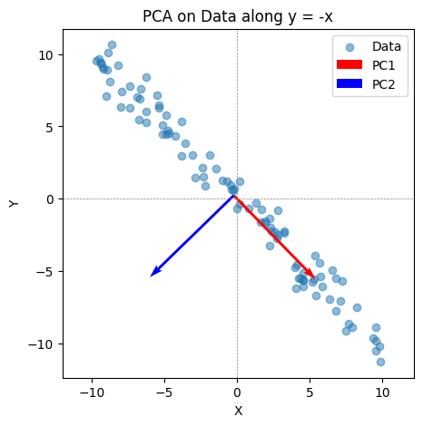
Consider trivial example in 2-dim, when we have data lying along the line \( y = -x\) plus some noise
We have \(X \in R^{n \times 2}\), with two features given by direction \((1, 0)\) and \((0, 1)\).
One would expect PC1 to give the direction \((1, -1)\).
Note the PC vector needs to have unit norm, giving roughly \((-0.7, -0.7)\)
import numpy as np
import matplotlib.pyplot as plt
from sklearn.decomposition import PCA

# Step 1: Simulate data along the line y = -x
n = 100  # Number of points
x = np.random.uniform(-10, 10, n)  # Random x values
y = -x + np.random.normal(0, 1, n)  # y = -x + noise

X = np.column_stack((x, y))  # Shape (n,2)

# Step 2: Perform PCA
pca = PCA(n_components=2)
pca.fit(X)

# Principal components
pc1 = pca.components_[0]  # First principal component
pc2 = pca.components_[1]  # Second principal component

print("First principal component:", pc1)
print("Second principal component:", pc2)

# Mean of data
mean = np.mean(X, axis=0)

# Step 3: Visualize the data and principal components
plt.figure(figsize=(5, 5))
plt.scatter(X[:, 0], X[:, 1], label="Data", alpha=0.5)

# Plot PC1 and PC2
plt.quiver(mean[0], mean[1], pc1[0], pc1[1],
            color='r', scale=3, label="PC1")
plt.quiver(mean[0], mean[1], pc2[0], pc2[1],
            color='b', scale=3, label="PC2")

plt.axhline(0, color='gray', linestyle='--', linewidth=0.5)
plt.axvline(0, color='gray', linestyle='--', linewidth=0.5)
plt.xlabel("X")
plt.ylabel("Y")
plt.title("PCA on Data along y = -x")
plt.legend()
plt.axis("equal")
plt.show()
First principal component: [ 0.6978726  -0.71622192]
Second principal component: [-0.71622192 -0.6978726 ]

