Importance Sampling#
This is referenced from Professor O.Deniz.Akyildiz’s Advanced Simulation course
When one wants to evaluate some integral \(\int \varphi(x) p(x) dx\) by using Monte Carlo integration, the variance reduction rate is \(O(1/N)\).
Problem is that we may not be directly able to sample from \(p\) (we may only have an unnormalized \(p\), or we are interested in some tail events, and outright MC has very low acceptance rate)
With IS, we obtain some weighted samples \(\{\mathsf{w}_i, X_i\}_{i=1}^N\), where the \(X_i\) are samples from some target \(q(x)\).
We can use the sample to evaluate any interested function \(\varphi(x)\) with respect to \(\pi(x)\):
This typically achieves variance reduction compared with basic MC integration, tho the variance decay rate is still \(O(1/N)\)
Tail Events#
Consider for example, for \(X \sim \mathcal{N}(0, 1)\):
Typical idea is to sample \(X_i \sim \mathcal{N}(0, 1)\), and if \(X_i > 4\), it is accepted as a sample. In this case, even if we sample \(N=10000\), we might still get 0 accpeted samples.
In this case we can use a propsal \(\mathcal{N}(6, 1)\), and weight each sample \(X_i\) by \(\frac{\mathcal{N}(X_i; 0, 1)}{\mathcal{N}(X_i; 6, 1)}\)
An implementation:
import numpy as np

rng = np.random.default_rng(26)
N = 10000
x_samples = rng.normal(6, 1, N)

xx = np.linspace(4, 20, 100000)

def p(x, mu, sigma):
    '''N(x|mu, sigma)'''
    return np.exp(-(x-mu)**2/(2*sigma**2))/(np.sqrt(2*np.pi)*sigma)

I = np.trapz(p(xx, 0, 1), xx) # Numerical computation of the integral
print('Integral of p(x) from 4 to infinity: ', I)

weights = p(x_samples, 0, 1)/p(x_samples, 6, 1)
IS_est = 1/N * np.sum((x_samples>4)*weights)
print('Importance sampling estimate: ', IS_est)
Integral of p(x) from 4 to infinity:  3.16712429751607e-05
Importance sampling estimate:  3.1925567492155485e-05
Self-normalizing IS#
When we are presented with unnormalized densities, IS won’t work.
Given \(\bar{p}(x)\) unnormalized, we don’t know the normalizing constant \(Z = \int \bar{p}(x) dx\) such that \(p = \bar{p}(x) / Z\) can be computed.
We want to compute
i.e. We can do two IS, one for numerator, one for denominator
Where \(W_i = \bar{p}(X_i) / q(X_i) \)
Say we want to estimate the mean of some unnormalized \(\bar{p}\), using propsal \(\mathcal{N}(0, \sigma_{\text{IS}}^2)\):
The SNIS algo is given by
Fix \(N, \sigma_{IS}\)
Sample \((X_1, \dots X_N) \sim \mathcal{N}(0, \sigma_{\text{IS}}^2)\).
Compute unnormalised weights \(W^{(i)} = \frac{\pi(X_{i})}{q(X_{i})}\).
Normalize weights \(w_i = \frac{W_i}{\sum_{j=1}^{N} W_j}\),
And we obtain the SNIS estimate of the posterior mean:
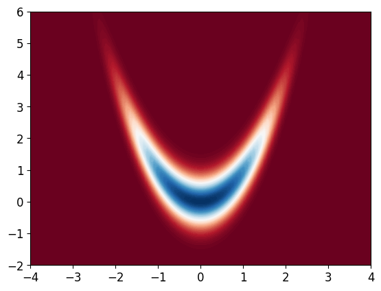
Consider the banana density, which is a numerically challenging density to integrate:
Since we cannot integrate it, we can’t normalize it. We first plot the density, and observe that the mean is around (0, 1)
import matplotlib.pyplot as plt

def Pi(x): # implementing the unnormalised density just for visualisation!
    return np.exp(-x[0]**2/10 - x[1]**2/10 - 2 * (x[1] - x[0]**2)**2)

def logPi(x):
    return - x[0]**2/10 - x[1]**2/10 - 2 * (x[1] - x[0]**2)**2

# we will only use log-density for the computations
x_bb = np.linspace(-4, 4, 100)
y_bb = np.linspace(-2, 6, 100)
X_bb, Y_bb = np.meshgrid(x_bb, y_bb)
Z_bb = np.zeros((100, 100))
for i in range(100):
    for j in range(100):
        Z_bb[i, j] = Pi([X_bb[i, j], Y_bb[i, j]])
plt.contourf(X_bb, Y_bb, Z_bb, 100, cmap='RdBu')
plt.show()

We are interested in estimating the mean of this density, i.e. compute \( \int x \; \pi(x) dx \)
We will do using a Gaussian propsoal \( q(x) = \mathcal{N}(x; 0, \sigma_{\text{IS}}^2) \)
Note the SNIS estimator is biased, but consistent (assymptotically unbiased)
In practice, to avoid numerical instability, we do
Fix \(N, \sigma_{IS}\)
Sample \((X_1, \dots X_N) \sim \mathcal{N}(0, \sigma_{\text{IS}}^2)\).
Compute unnormalised log weights
Remove most extreme likelihood
Equivalent to setting all weights as a ratio of the largest weight:
Normalize weights (log-sum-exp)
$\( w_i = \frac{e^{\log W_i}}{\sum_{j=1}^{N} e^{\log W_i}} = \frac{W_i}{\sum_{j=1}^{N} W_j} \)$,
sig_     = 5 # standard deviation of the proposal

def logq(x, sig): # log-density of the proposal
    return - x[0]**2/(2 * sig**2) - x[1]**2/(2 * sig**2) - np.log(2 * np.pi * sig**2)

# Self-normalised importance sampling
def SNIS_banana(N, sig):
    x_samples = rng.normal(0, sig, (N, 2)) # N 2D samples from the proposal
    logw = np.zeros(N) # log-weights
    for i in range(N):
        logw[i] = logPi(x_samples[i, :]) - logq(x_samples[i, :], sig)
    logw = logw - np.max(logw) # to avoid numerical issues (look up this trick)
    w = np.exp(logw)/np.sum(np.exp(logw)) # normalising the weights
    return np.sum(w[:, np.newaxis] * x_samples, axis=0)

N = 100000
phi_SNIS = SNIS_banana(N, sig_  )
print('estimated mean:', phi_SNIS)
estimated mean: [-0.00549162 0.90488818]
Sampling from Bayesian Posterior#
Under a Bayesian setting, let us take our \(\pi(x)\) as a prior.
Assume we have observed \( y = 1\). Let the likelihood be
where \(H = [1, 0]\). i.e. Only the first dimension of the state \(x\) is observed in the likelihood
Let \(\sigma = 0.01\) (assume we have observed \(y\) with a very small variance)
We wish to sample from the posterior
We will still use proposal \(q = \mathcal{N}(x; 0, \sigma_0^2 I)\).
So the importance weights:
def loglik(y, x, sig):
    H = [1, 0]
    return -(y - H @ x)**2/(2 * sig**2) - np.log(sig * np.sqrt(2 * np.pi))

sig = 0.01 # standard deviation of the likelihood
y = 1 # observation

sig_q = 1 # standard deviation of the proposal

N = 10000
# sample from q
x = rng.normal(0, 1, (2, N)) # 2 x N matrix (2 dimensional, N samples)

# compute logW
logW = np.zeros(N)
for i in range(N):
    logW[i] = (loglik(y, x[:, i], sig)) + logPi(x[:, i]) - logq(x[:, i], sig_q)

logW = logW - np.max(logW)
w = np.exp(logW)/np.sum(np.exp(logW))

mean = np.sum(w * x, axis=1)

print(mean)
[0.99824318 0.99655733]
To measure the performance of a SNIS estimator, one can use the effective sample size (ESS), as a function of the N weights
def ESS(w): # To measure sample quality
    return 1/np.sum(w**2)

print("ESS: ", ESS(w))
ESS: 39.52618998441565
Resampling#
We now have the weighted samples \(\{\mathsf{w}_i, X_i\}_{i=1}^N\).
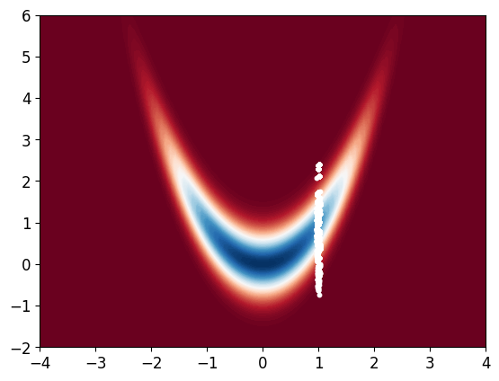
We want to plot the scatterplot of posterior samples, but we cannot do so with \(X_i\), as they are samples from \(q\) without the weights. We may wish to have an unweighted sample from the posterior.
Note with weighted samples, not only can we generate the estimated mean \(\sum w_i X_i\), we can also build an empirical estimate of the target density
Which is basically the discrete distribution that assigns probability \(w_i\) at \(X_i\), and 0 otherwise
We can obtain an unweighted sample from the same measure, by sampling i.i.d from \(\tilde{\pi}^{N}\),
i.e., sampling particles \(\{ x^{(i)} \}_{i=1}^{N}\) with replacement from \(\{\mathsf{w}_i, X_i\}_{i=1}^N\).
with probabilities \(\{ \mathsf{w}_i \}_{i=1}^{N}\).
This means for \(X_i\) that corresponds to high \(\mathsf{w}_i\), it will simply be sampled for multiple times (with replacement) from our resample, and would represent a proportion of \(\mathsf{w}_i\) in the new sample
# resample N samples
x_resampled = np.zeros((2, N))
for i in range(N):
    x_resampled[:, i] = x[:, rng.choice(N, p=w)]
    # rng.choice chooses an index from 0 to N-1 with probability w

# now we resampled N samples from this sample set,
# plotting them will give us an approximation of the posterior

# plot resampled samples
x_bb = np.linspace(-4, 4, 100)
y_bb = np.linspace(-2, 6, 100)
X_bb, Y_bb = np.meshgrid(x_bb, y_bb)
Z_bb = np.zeros((100, 100))
for i in range(100):
    for j in range(100):
        Z_bb[i, j] = Pi([X_bb[i, j], Y_bb[i, j]])
plt.contourf(X_bb, Y_bb, Z_bb, 100, cmap='RdBu')
plt.scatter(x_resampled[0, :], x_resampled[1, :], s=10, c='white')
plt.show()

